MGSLG ICTCFT. (2017). Adding column totals (CC BY-SA)
View
Video Transcript
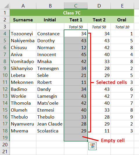
- Using the mouse, select the cells in the first column in which the first test marks have been inserted, that is from C4 downwards (click the left mouse button and keep it pressed in while you drag the mouse down the column or row.
- You will know if you have been successful as the column turns light blue once selected.
- Continue down to the last value and include one extra empty cell. It is in this last cell that the answer will appear.

- With the column selected press the ‘Σ’ button at the top of the screen (Autosum). The total of the column will now appear in the extra cell.
- Type ‘Total’ in the same row but in column A.
- Make it both the label and value in that row bold.
- You can also find out the sum of a series of cells by typing in the following formula where you want the answer to appear, =SUM(c4:c29).
- The formula means: use the function SUM to add the contents of the column C from Row 4 to Row 29.
- If your class is bigger or smaller than 25 you will need to adjust the second row number to the last person in your workbook.
- Notice the formula appears in the cell-editing field at the top of the screen. Should you make a mistake and wish to correct the formula, select the cell in question and then click inside this field.
- You can then edit the formula as you wish.
Last modified: Wednesday, 28 September 2022, 10:32 AM